7 Accuracy and Sub- / Super-pixel analysis
7.1 Summary
This week we focus on measuring the accuracy of the classification, and object-based and sub-pixel analysis.
7.1.1 Accuracy
7.1.1.1 Accuracy Measures
The accuracy measures for remote sensing (and machine learning in general) is based upon comparing the positive / negative classifications to what the values actually were. The four possibilities that are considered can be organised as the following table.
| Actually Positive | Actually Negative | Accuracy Measure | Error | |
|---|---|---|---|---|
| Positively Classified | True Positive | False Positive | User’s Accuracy (Precision) | Commission Error |
| Negatively Classified | False Negative | True Negative | Negative Predictive Value | False Ommision Rate |
| Accuracy Measure | Producer’s Accuracy (Recall) | True Negative Rate | ||
| Error | Omission Error | False Positive Rate |
The producer’s accuracy is the rate of pixels correctly positively identified to the ground truth data. This shows the accuracy from the producer’s point of view, calculating the correctly classified data.
\[ \text{Producer's Accuracy} = \frac{\text{TP}}{\text{TP}+\text{FN}} \]
On the other hand, the user’s accuracy defines the ratio of correctly identified pixels within the values that are classified as positive. This is the accuracy from the user’s perspective, as the classified data is taken as the dividend.
\[ \text{User's Accuracy} = \frac{\text{TP}}{\text{TP}+\text{FP}} \]
The overall accuracy is the rate of correctly identified (positively or negatively) cells.
\[ \text{Overall Accuracy} = \frac{\text{TP}+\text{TN}}{\text{TP}+\text{FP}+\text{TN}+\text{FN}} \]
From this overall accuracy measures, a widely used but inconsistent coefficient, the kappa coefficient, can be calculated. This values compares the accuracy to a randomly classified value. When \(p_o\) is the overall accuracy and \(p_e\) the expected accuracy when classified randomly, the kappa coefficient \(\kappa\) can be calculated as:
\[ \kappa = \frac{p_o-p_e}{1-p_e} \]
The inconsistency in this coefficient is argued by Foody (2020), because there is a range of values that can be taken by the kappa coefficient, and it is difficult to interpret these values.
7.1.1.2 Trade-offs
The producer’s accuracy (precision) and the user’s accuracy (recall) is a trade-off: if we wanted to improve the producer’s accuracy, we will lower the threshold to increase the number of positively identified pixels. This will lead to more false positive values as well, thus causing a decrease in the user’s accuracy. Therefore, there is a need to consider both of these values to determine a good balance between precision and recall. The F-1 score is one of these measures, combining these two factors (Wilber 2022a).
\[ F_1 = \frac{2 \cdot \text{PA} \cdot \text{UA}}{\text{PA} + \text{UA}} = \frac{{\text{TP}}}{\text{TP} + \frac{1}{2} \left( \text{FP} + \text{FN} \right)} \]
Another measure is the area under the ROC (Receiver Operating Characteristics) curve. The ROC curve is an indicator of the classification characteristics with false positive rates on the x axis and true positive rates on the y axis.
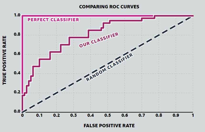
The area under this curve (AUC) can be a measurement of the classification method, where a larger area indicates a better classification technique. A random classification will have an AUC of 0.5, and a perfect classification will have a value of 1.
7.1.1.3 Testing the accuracy
As with other machine learning, the training data and testing data must be different datasets. The following is a list of common procedures to generate training and testing data.
- Train-test split: leaving a certain percentage of the dataset for testing, and not use for training
- Cross-validation: split the dataset into \(k\) parts, leave one segment at a time to test with model trained with the remainder
- Leave one out cross-validation: an extreme example of the above, just leaving one observation at a time
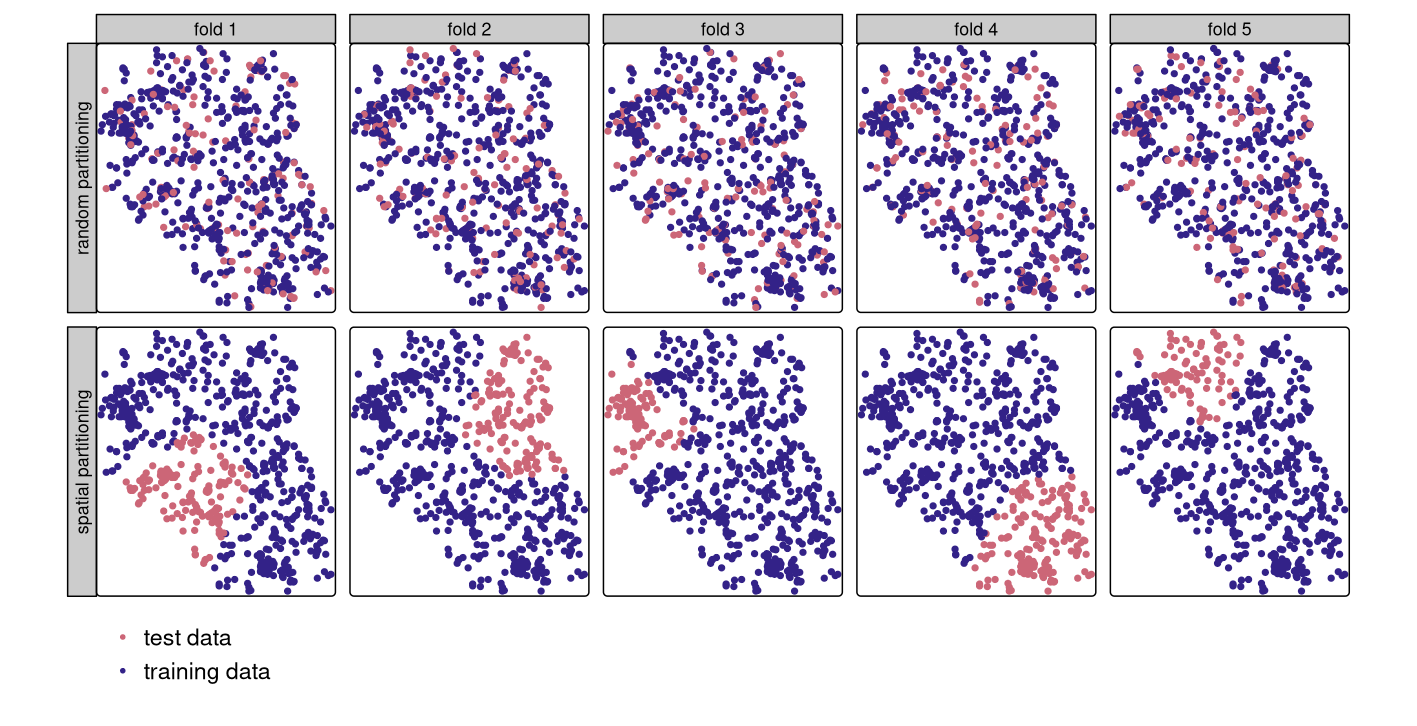
Spatial autocorrelation is an important factor that must be considered in this process, but the above mentioned techniques all do not consider this when applied naively. Having the testing data very close to the training data is an inappropriate setting, as it is very likely to have the similar characteristics as the training dataset. A spatial cross-validation considers the spatial distribution of the training and testing datasets, taking a spatial subset of the dataset to keep for testing.
7.1.2 Object-based analysis
Instead of considering a single pixel at a time, the idea of object-based analysis is to take a group of cells (superpixels) clustered by their similarity or difference. A common way to achieve this is the Simple Linear Iterative Clustering method, where each cell is classified to the nearest centroid, with the distance considering both spectral and spatial distance. One simple example of this is:
\[ d = \sqrt{\left( \frac{d_c}{m} \right)^2 + \left( \frac{d_s}{S} \right)^2} \]
where - \(d_c\) spectral distance - \(m\) compactness parameter - \(d_s\) spatial distance - \(S\) interval between initial clusters
Improved models for considering other distance measures (other than Euclidian) are created and implemented under the Supercells package.
The centroid is recalculated after the reclassification, and the process is iterated over multiple times (usually 5 - 10) to achieve the final output of classifications.
Classification algorithms are overlaid for each of the clusters rather than focusing on individual clusters.
7.1.3 Sub-pixel analysis
In contrast, sub-pixel analysis tries to identify the mixture within an area represented by a single pixel.
Sub-pixel analysis assumes the data a pixel obtains is a combination of multiple pure land covers - endmembers - mixed in a certain ratio, as illustrated below.

When the pixel values for each of the endmembers are observed as \(p_{i\lambda}\), the mixed spectrum \(p_{\lambda}\)can be broken down as
\[ p_{\lambda} = \sum_i{\left( p_{i\lambda}\cdot f_i \right)}+e_\lambda \] where \(f_i\) is the fractional cover for each of the endmembers, and \(e_{\lambda}\) being the model error.
A common model used in the urban context is the VIS model, where the endmembers Vegetation, Impervious surface, and Soil are considered.
Under this model, when the pixel values for each of the \(k\) bands are expressed as
\[ p = \begin{bmatrix} p_1 \\ p_2 \\ \vdots \\ p_k \end{bmatrix} \]
the fractional cover for each endmember can be calculated as shown below.
\[ \begin{gather} \begin{cases} p_{\lambda} = \begin{bmatrix} p_V & p_I & p_S \end{bmatrix} \begin{bmatrix} f_V \\ f_I \\ f_S \end{bmatrix} \\ f_V + f_I + f_S = 1 \end{cases} \\ \\ \therefore \begin{bmatrix} p_{\lambda 1} \\ p_{\lambda 2} \\ \vdots \\ p_{\lambda k} \\ 1 \end{bmatrix} = \begin{bmatrix} p_{V1} & p_{I1} & p_{S1} \\ p_{V2} & p_{I2} & p_{S2} \\ \vdots & \vdots & \vdots \\ p_{Vk} & p_{Ik} & p_{Sk} \\ 1 & 1 & 1 \end{bmatrix} \begin{bmatrix} f_V \\ f_I \\ f_S \end{bmatrix} \\ \Leftrightarrow \begin{bmatrix} f_V \\ f_I \\ f_S \end{bmatrix} = \begin{bmatrix} p_{V1} & p_{I1} & p_{S1} \\ p_{V2} & p_{I2} & p_{S2} \\ \vdots & \vdots & \vdots \\ p_{Vk} & p_{Ik} & p_{Sk} \\ 1 & 1 & 1 \end{bmatrix}^{-1} \begin{bmatrix} p_{\lambda 1} \\ p_{\lambda 2} \\ \vdots \\ p_{\lambda k} \\ 1 \end{bmatrix} \end{gather} \]
A limitation of this method can lie in identifying the endmembers, where it requires the existence of a pixel wit a ‘pure’ land cover - which may not be obvious.
7.2 Applications
Applications of accuracy measures are often used for comparisons between models. Rozenstein and Karnieli (2011) explores the use of multiple classification models to identify the land cover to create a database of land cover for Israel. They have also conducted a post-classification accuracy improvement procedure to enhance their results of classification. The confusion matrix, producer’s and user’s accuracies, and the kappa coefficient was used to anlayse the accuracy of each method, concluding the hybrid approach of unsupervised and supervised learning methods have achieved the highest accuracy. One interesting point made is that the desired accuracy measure of 85% introduced in past research is not always achieved when informing planning decisions, including the outcomes of this research.
Roberts et al. (2017) explores the need for cross-validation techniques that take into consideration not only spatial autocorrelation but also having other underlying structures within the dataset. Creating blocks in the spatial context, temporal blocking, and leaving out individual observations are considered as potential methodologies to prevent overfitting and underestimating the errors of the machine learning model. This study does point out, however, that extrapolation errors emerge as new problems and this requires consideration as well - in the spatial context, the shape of each ‘block’ is suggested to impact this error.
These research papers show the two aspects of accuracy in literature - the first paper is an example of accuracy used as part of the data pipeline that is helping the assessment of multiple models to serve a purpose, and the second model is the exploration of methodology that addresses and assesses accuracy. The first model uses the kappa coefficient - which is accused of being inconsistent but still being widely used - is an example of how this area is still under development and improvements must be made. The second paper shows that spatial autocorrelation is one of the many aspects that must be considered, which is an important thing to keep in mind.
7.3 Reflections
This week we have observed the assessment of accuracy in remote sensing and procedures to improve and correctly handle this field.
Important messages to take home are:
- just because one measurement is widely used does not mean it is an appropriate one - we must consider whether the coefficients that we have are actually valid
- spatial autocorrelation must be considered when conducting classification - this is a new perspective that is unique when we are to handle spatial data in particular
Even though this part does is not always our main interest, it is an important phase within our data processing pipeline that seeks to achieve other goals. Since accuracy is an inevitable aspect of academic research, we must keep in mind how to analyse the data correctly and with precision.